Analysing seasonal patterns in TourMIS
The picture is clear in everyone’s mind: European cities are now packed with tourists, the streets full of people holding a map in one hand and a camera in the other, queues at the entrance of the main attractions, hotel rooms fully booked and the traffic congested. But as soon as the Christmas Season is over, the number of visitors can rapidly diminish making these same places look like ghost towns – until the next wave.
\n
Every city in Europe experiences a certain degree of demand seasonality, an undesirable characteristic of tourism, which prevents the optimal use of a destination’s facilities and resources. Empty hotels during the off-peak season are only the most obvious effect: seasonality has an impact on all aspects of supply-side behaviour in tourism, including marketing, pricing, cash-flow, the labour market and attraction of investment capital. A variety of measures to even out the demand pattern, ranging from the organisation of the event calendar to differentiating the market mix, can be taken by tourism managers. Obviously, these interventions require insight into the phenomenon – to identify suitable and effective steps and to prioritize them correctly within the overall tourism policy.
\n
\n
With the aim of supporting the decision-making and planning process of tourism managers, TourMIS provides a tool to perform analyses of seasonality. The function is available at the www.tourmis.info web site and can be reached by clicking on the “Nights & arrivals” link in the “City tourism in Europe” menu and selecting “monthly data”. A click on the “Assessing seasonality” link opens a drop down menu where the destination of interest can be selected; next, the type of time series (arrivals or overnights), the source market and the year of reference can further be specified. This option is important to obtain target-oriented results. In fact, investigating the aggregate flow of visitors to a destination over one year is more appropriate to deciding where an event should be placed on the calendar, while an analysis of the overnights distribution for a specific market is more meaningful when making a decision about a marketing campaign.
\n
\n
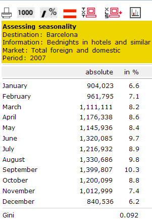
The outcome of the query is presented in tabular form where both the figures (absolute and relative value) and the seasonal indicator (the “Gini coefficient[1]”) for the specified destination are displayed (table on the left- hand side in fig. 1).
\n
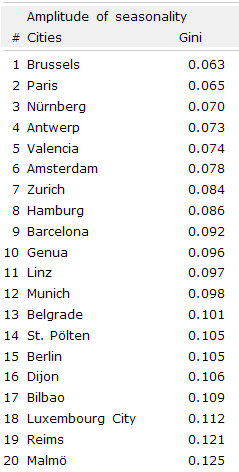
The table at the bottom of the web page (the right-hand column in fig. 1) simplifies comparisons with other European cities, since it displays the value of the Gini coefficient (amplitude of seasonality) in ascending order.
\n
At a glance, the Gini coefficient reveals to what extent the destination is affected by seasonality (the amplitude of seasonality). A value approaching 0 corresponds to an evenly distributed series, and a value approaching 1 relates to a highly concentrated distribution. Figure 2 illustrates distributions of the extreme values, which the Gini coefficient can have, and compares them with two real cases. Zurich’s value of the Gini coefficient (0,087) reflects an almost equally distributed series of arrivals.
\n
Similarly, Dubrovnik’s high value (0.511) reflects a demand concentrated in a few months.
\n
Back to the example in figure 1, Barcelona can be assessed as a destination with a rather smooth pattern.
\n
\n
To conclude, TourMIS’ seasonal indicator can be used to perform a number of worthwhile analyses, such as
\n
\n
• assessing the seasonal amplitude of demand for a destination,
\n
• assessing the seasonal amplitude of demand for a destination from specific geographical markets,
\n
• monitoring how seasonal amplitude changes over time and
\n
• benchmarking seasonal amplitude in relation to other cities in Europe,
\n
\n
This should encourage managers to perform longitudinal and cross-destination analyses of seasonality, whose time horizon goes beyond the beginning of the next season.
\n
\n
\n
\n
[1] The Gini coefficient is a measure of the inequality of a distribution, named after the Italian statsitician Corrado Gini, who first applied it (Variabilitá e mutabilitá . Economics and Law Studies, Vol. Bologna: Cuppini).
\n
\n
\n
\n
\n
\n

\n